On this page

What is High-Cardinality
Cardinality, as defined by Wikipedia, is a mathematical term used to quantify the number of elements in a set. For example, the cardinality of a finite set A = {a, b, c} would be 3. While the concept of cardinality also extends to infinite sets, we won't delve into that area here since our primary focus for today is centered around the field of computer science.
In the context of databases, cardinality does not have a strict definition. What is generally agreed is that cardinality is used to measure the number of different values contained in a data column. For example, in a table recording User info, there are usually UID, Name and Gender columns. Obviously, the UID has the highest cardinality because each user is assigned a unique ID. The Name also has a high cardinality, but since there may be users with the same name, it is not as high as UID. The number of values in the Gender column is the least. So in this example of a user table, the UID column can be called high-cardinality and Gendercan be called low-cardinality.
If further subdivided into the field of time series databases, cardinality often specifically refers to the number of the timeline. Let's take the application of time series databases in the Observability field as an example. A typical scenario is the recording of the response time for API services. When we want to monitor the response time of various API services, it often entails measuring the time taken by each access interface for different instance API services. This process usually includes two labels: API Routes and Instances. If there are 20 interfaces and 5 instances, the cardinality of the timeline is (20 + 1) x (5 + 1) - 1 = 125 (The reason for adding +1 here is to consider the response time of all interfaces for a specific instance, or a certain interface across all instances.) Though the number does not seem large, keep in mind that the operator is multiplication, so if the cardinality of a label is high, or if a new label is added, it will cause the cardinality of the timeline to increase exponentially.
Why it matters
We know that for relational databases such as MySQL that we are most familiar with, they usually contain high-cardinality columns such as ID, Email, Order_number, etc. However, it is rare to hear that such data modelling causes problems. The truth is, in the field of OLTP, high cardinality often doesn't pose a problem, but in the realm of time-series, due to the data model, it frequently causes issues. Before we delve into the subject of time-series, let's first discuss what a high-cardinality dataset means.
In my view, a high-cardinality dataset means a large amount of data. For a database, an increase in the volume of data will inevitably affect writing, querying, and storage. Specifically, indexes are most significantly impacted during writing operations.
High-Cardinality in traditional databases
In relational databases, the B-tree data structure is the most commonly used data structure to construct indexes. In general, the complexity of inserting and querying is O(logN), and the space complexity is O(N), where N is the number of elements, or what we refer to as cardinality. While a larger N may have some impact, it is not too significant since the complexity of insertion and querying is logarithmic.
So it seems that high-cardinality data does not has a significant impact. Since the selectivity of indexes on high-cardinality data is stronger than that of indexes on low-cardinality data, high-cardinality indexes can filter out a majority of data that does not meet the query conditions through only one query condition, reducing the overhead of disk I/O. In database applications, it is necessary to minimize disk and network I/O overhead. For example, when executing select * from users where gender = 'male';, the resulting dataset is usually large, requiring huge disk and network I/O. However, using such a low-cardinality index alone is not particularly meaningful in reality.
So in most cases, high-cardinality does not tend to be an issue in traditional OLTP databases.
High-Cardinality in time-series database
Then why is it so different when it comes to time-series databases and how can high-cardinality data columns cause problems?
In the field of time-series databases, the core of data modeling and engine design lies on the timeline. As mentioned earlier, the issue of high-cardinality in time-series databases refers to the size of timelines. The size is not just the cardinality of one column, but the product of the cardinalities of all label columns, so it increases drastically. This can be understood as in common relational databases where high cardinality is isolated in a particular column, the data scale increase lineally, while in the time-series databases, the high-cardinality is a product of multiple columns, it increases nonlinearly.
Let's take a closer look at how high cardinality timelines are created in time-series databases.
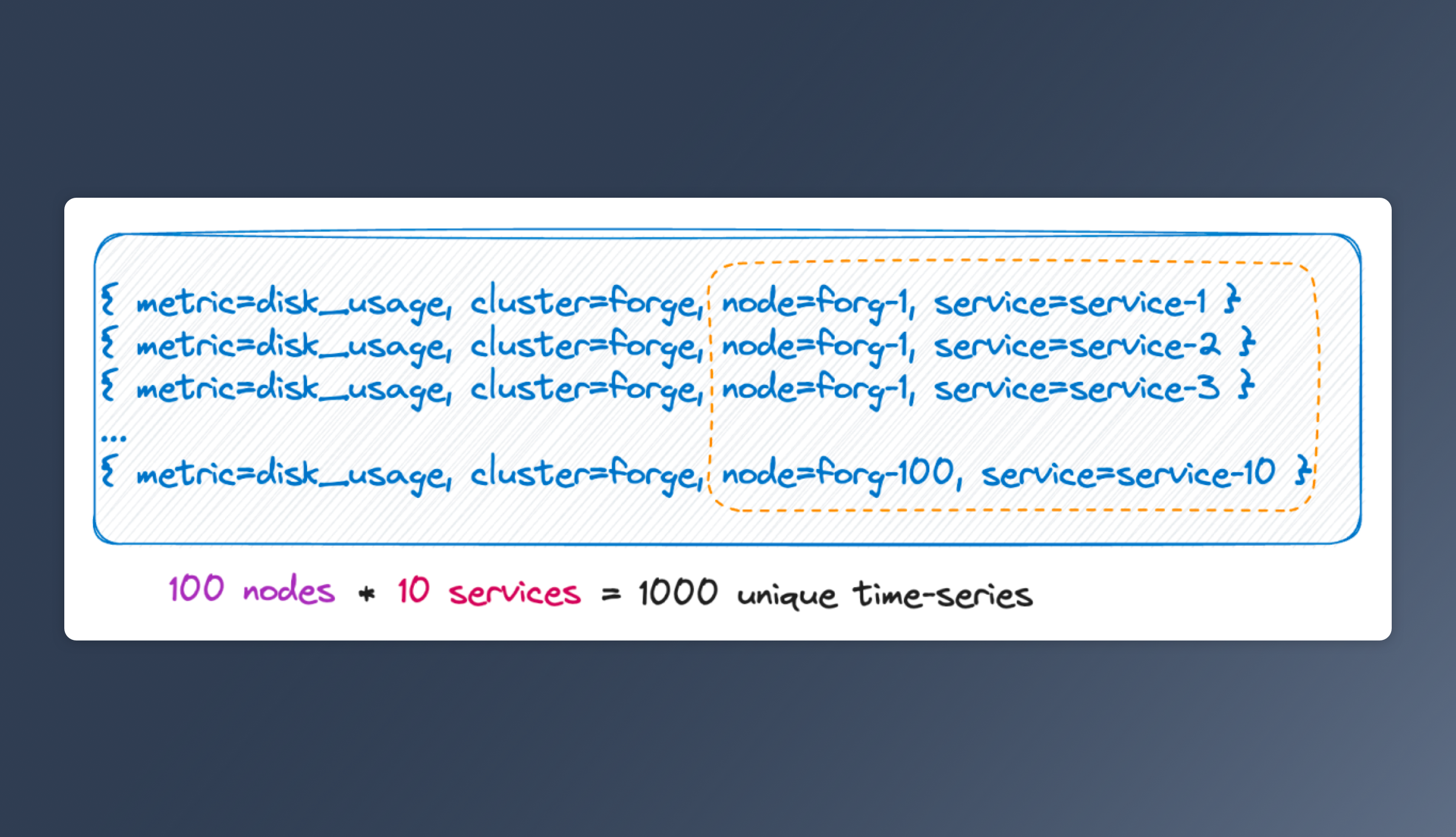
Time-series
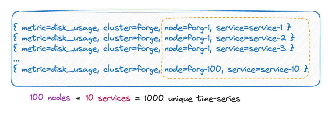
We know that the number of timelines actually equals the Cartesian product of all the cardinalities of labels. As shown in the figure above, the number of timelines is 100 * 10 = 1000. If you add 6 more labels to this metric with 10 value options for each label, the number of timelines would be 10^9, which is astonishingly huge.
Labels with infinite value
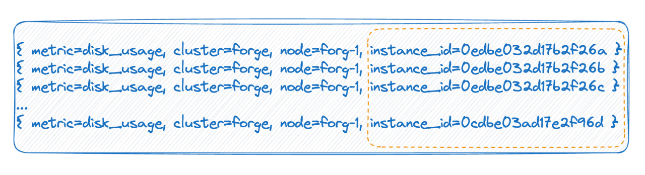
In the second scenario, within a cloud-native environment, every pod possesses a unique ID. Upon each restart, the existing pod is removed and subsequently reconstructed, consequently creating a new ID. This process leads to an extensive amount of label values, and with every complete restart, the timeline count doubles.
These two scenarios primarily account for the high-cardinality observed in the time-series database.
How time-series databases store data
Now that we know how high-cardinality is generated, to understand what problems it may cause, we also need to know how mainstream time-series databases organize data.
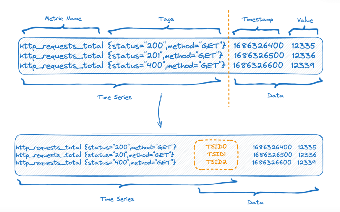
The upper part of the figure represents the way the data looks before it is written, while the lower part shows how the data is logically arranged after flushing to storage. On the left side, you can see the time-series section (the index data), and on the right side, you can observe the actual data.
Each time-series is associated with a unique Time-Series ID (TSID), which serves as a link between the index and the data. Those who are familiar with this concept might have recognized that the index used here is actually an inverted index.
Let's take a closer look at the representation form of the inverted index in memory:
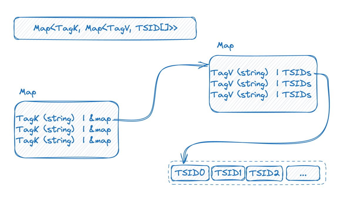
The above figure depicts a double-layer map. The outer layer first locates the inner map using the label name as a key. Inside the inner map, the key (K) represents the label value, while the value (V) is a set of TSIDs that contain the corresponding label value.
Up to this point, considering the information provided earlier, it becomes evident that the size of the double-layer map increases with the higher cardinality of the time series data.
Grasping the index structure, we can now try to understand how high-cardinality causes problems.
To attain high throughput writing, it is preferable to maintain the index in memory. However, when dealing with high-cardinality data, the index can become inflated, exceeding the memory capacity. As a result, the index cannot be fully accommodated in memory, necessitating swapping it to the disk. This situation leads to a significant number of random disk Input/Output (IO) operations, which adversely impacts the write speed.
Now let's move our eyes to the query operation. By examining the index structure, we can easily understand the query process for the condition where "status = 200" and "method = get.". The process begins by locating the map associated with the key status to access the inner map. From this inner map, we retrieve all TSID sets linked to the index key 200. Similarly, we follow this approach to find the next condition. Finally, we fetch the actual data using the TSIDs from the intersection of the TSID sets, resulting in the desired query results.
The core problem here is that, since data is organized along the timeline, one needs to get the timeline first before finding the data according to the timeline. So the more timelines involved in a query, the slower the query will be.
How to solve it
If our analysis is correct, that is, we know the cause of the high-cardinality issue in time-series databases, then there will always be some ways to solve it. Let's look at the cause of the problem:
- Data modelling level: The index maintenance and query challenge caused by C(L1) * C(L2) * C(L3) * ... * C(Ln).
- Technical level: The data is organized according to the timeline, so you first need to get the timeline, and then find the data according to the timeline. The more timelines, the slower the query.
Now let me suggest some solutions separately from these two perspectives:
Optimize from data modelling:
#1 Remove unused labels
We often inadvertently set some unnecessary fields as labels, which leads to timeline bloating. For example, when we monitor the server status, we often have instance_name and IP. In fact, these two fields do not need to be labels, having one of them is likely enough, and the other can be set as an attribute.
#2 Model Query Fit
Take the monitoring of sensors in the IoT as an example, assuming we have three labels at the beginning:
- 100,000 devices
- 100 regions
- 10 types of devices
If these are modelled into a single metric in Prometheus, it would result in 100,000 * 100 * 10 = 100 million timelines.
Now, let's pause here and take a moment to reflect on the real-world situation: would the query be requested in this manner? For instance, will there be a business case to query the timeline of a certain type of device in a certain location? This doesn't seem quite reasonable because once a device is specified, its type is also determined. Therefore, these two labels may not need to be queried together, and we can split one metric into two:
- metric_one:
- 100 regions
- 10 types of devices
- metric_two:(Assuming a device might change regions to collect data)
- 100,000 devices
- 100 regions
This would lead to approximately 10010 + 100,000100 ~ 10.1 million timelines, which is 10 times less than the previous calculation.
#3 Isolate high cardinality
Of course, if your data model is highly consistent with the query, but you still can't reduce the timeline due to the large scale of the data, then I suggest to put all the services related to this core indicator on a separate, high-performance machine.
From the technical view:
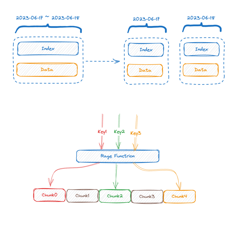
- The first solution is vertical partitioning, which is adopted by most of the mainstream time-series databases. They partition the index by time, because if you don't do this partitioning, your index will get bigger and bigger when continuously ingesting data, and finally, it will not be able to store into the memory. If partitioning by time, you can swap old index chunks to disk or even remote storage, so at least writing will not be affected.
- Opposite to vertical partitioning is horizontal partitioning, which uses a sharding key, typically a label that most frequently appears in query predicates, to perform range or hash partitioning based on the values of these labels. This solution leverages a distributed divide-and-conquer approach to address the bottleneck on a single machine. The drawback is that if your query condition does not contain the sharding key, most likely, you cannot push down the operator and can only retrieve the data to the uppermost level for computation.
The above method is a typical solution, which can only alleviate the problem to a certain extent, but cannot systematically solve the problem.
The next two solutions are not so conventional, they are the ideas that GreptimeDB is trying to explore for your reference:
- We might need to ask ourselves the question, do time-series databases really need an inverted index? If we look at popular TSDBs for example, TimescaleDB uses a B-tree index, and InfluxDB_IOx also does not use an inverted index. For high-cardinality queries, if we use some pruning optimization with partition scanning, which is commonly used in OLAP databases, combined with min-max indices, would that provide better performance?
- As for asynchronous intelligent indexing, in order to asynchronously build the most suitable index to speed up the query, we must first collect and analyze behaviors and find patterns from each of the user's query. For instance, for labels that appear at a very low frequency in the user's query scenarios, we choose not to create an inverted index.
Because the inverted index is built asynchronously, it does not affect the writing speed at all for both of the two methods above.
If we then look at the query, because time series data have a time attribute, the data can be bucketed according to the timestamp. We do not index the most recent time bucket - the solution is to use a brute force scan, combined with some min-max type indices for pruning optimization. This solution makes it possible to scan tens of millions or even hundreds of millions of rows in seconds!
When a query comes in, you could first estimate how many timelines it involves; If there are only a few, use the inverted index. If there are many, use the scan + filter method.
We are still continuously exploring around these ideas, and they are not yet perfect.
Conclusion
High cardinality is not always an issue, sometimes it is inevitable. What we need to do is to build our own data model based on business requirements and the features of the technical tools used. You may be wondering what if the tool has certain limitations? For example, Prometheus by default, adds indexes for each label under each metric, which is not a big problem on a single-machine, but it is inadequate for large-scale data. GreptimeDB is committed to creating a unified solution for both single-machine and large-scale use cases. We are also exploring technical attempts to solve problems of high cardinality and welcome everyone to discuss together.


