
On this page

Background
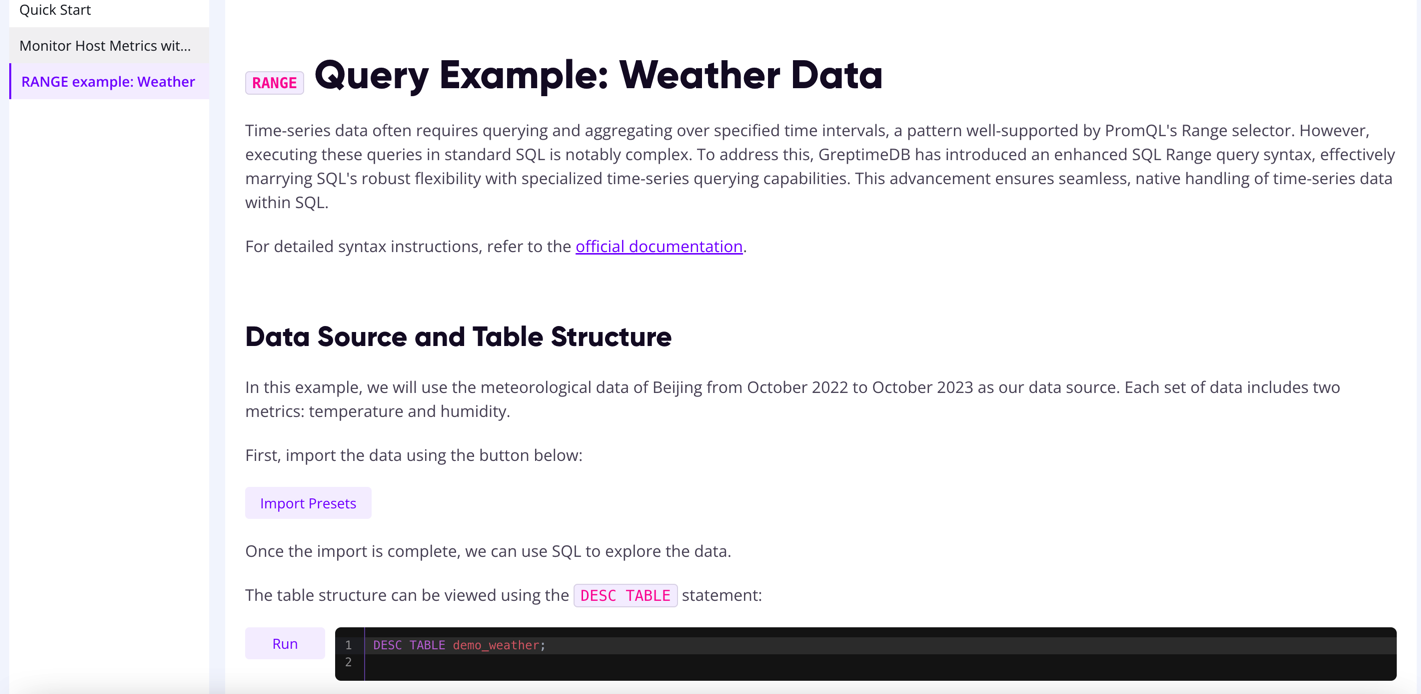
Time-series data often requires querying and aggregating over specified time intervals, a pattern well-supported by PromQL's Range selector. However, executing these queries in standard SQL is notably complex. To address this, GreptimeDB has introduced an enhanced SQL Range query syntax, effectively marrying SQL's robust flexibility with specialized time-series querying capabilities. This advancement ensures seamless, native handling of time-series data within SQL.
Explore Range Queries with SQL on GreptimePlay
Our interactive documentation for range queries is now officially available on GreptimePlay!
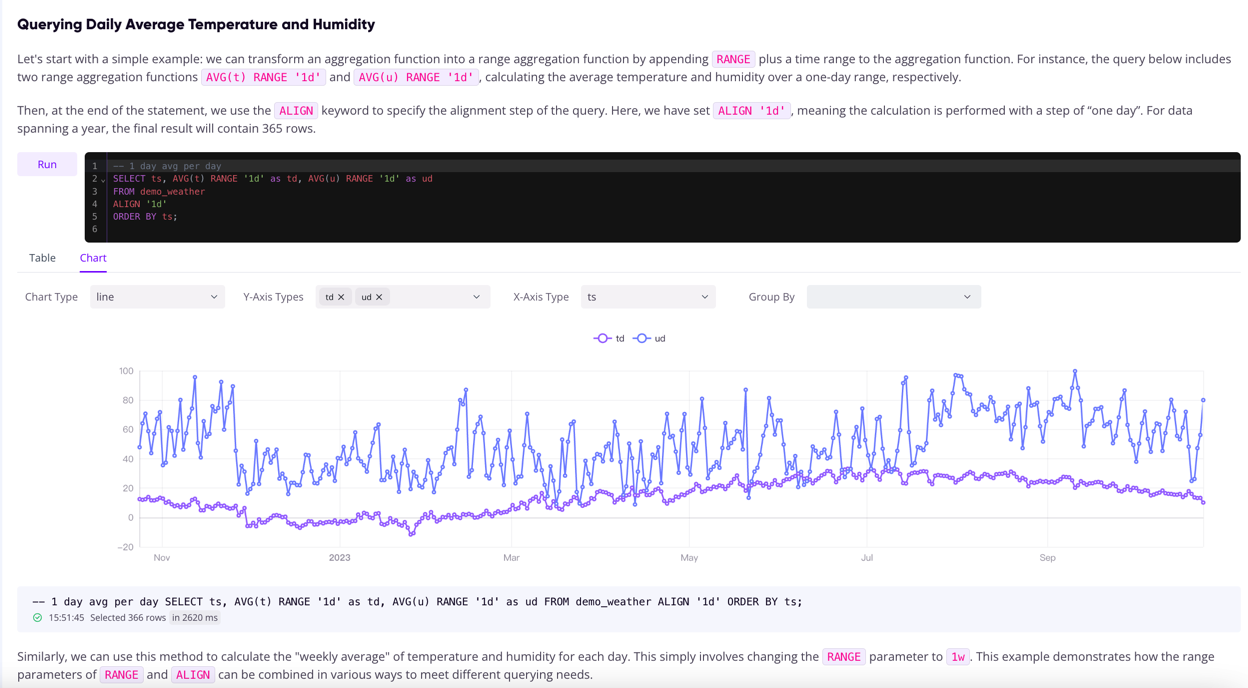
You can delve into various query techniques through a daily example using SQL and receive immediate, visualized feedback. Dive into the world of dynamic data querying on GreptimePlay today!
Example
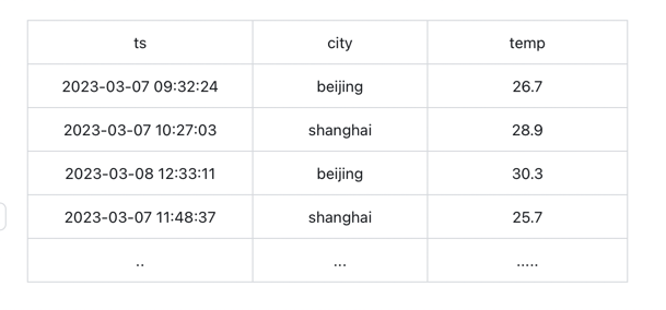
Let's illustrate the Range query with an example. The following temperature table records the temperatures in different cities at various times:
For the given scenario, where we want to query the daily and weekly average temperatures in Beijing up to May 2, 2023 (timestamp 1682985600000), with a fallback to use linear interpolation to estimate query values for missing data.
To conduct these two queries in PromQL, it is structured with a day as the step size. For the daily average temperature, we aggregate data over each day. For the weekly average, we extend this aggregation to a week-long period, calculating the average for each week. Additionally, to align our query with the specific timestamp of 1682985600000, we use the @ operator in PromQL. This aligns the query execution time exactly to the given timestamp, ensuring accurate and relevant data retrieval for the specified period.
The final query looks like this:
sql
-- Daily average temperature
avg_over_time(temperature{city="beijing"}[1d] @ 1682985600000) step=1d

-- Weekly average temperature
avg_over_time(temperature{city="beijing"}[7d] @ 1682985600000) step=1d
However, the above query has some issues: PromQL emphasizes on data querying but struggles with handling missing data points, i.e., smoothing the queried data. Though PromQL has a Lookback delta mechanism (see this article for more details), which uses old data to replace missing data points, this default behavior might not be desirable for users under certain circumstances. Due to the existence of the Lookback delta mechanism, aggregated data might carry some old values. And it is challenging for PromQL to precisely control data accuracy. Furthermore, PromQL does not have an effective method for data smoothing, as our requirement mentioned above.
From a traditional SQL perspective, since there is no such Lookback delta mechanism, we can precisely control the scope of our data selection and aggregation, allowing for more accurate queries.
The query here essentially aggregates data daily and weekly. For daily average temperatures, we can use the scalar function date_trunc, which truncates timestamp to a certain precision. We use this function to truncate time to a daily unit and then aggregate the data by day to get the desired results.
sql
-- Daily average temperature
SELECT
    day,
    avg(temp),
FROM (
    SELECT
        date_trunc('day', ts) as day
        temp,
    FROM
        temperature
    WHERE
        city="beijing" and ts < 1682985600000
)
GROUP BY day;
The above query roughly meets our needs, but there are issues with this type of query:
Complicated to write with the subqueries required;
This method can only calculate daily average temperatures, not weekly averages. In SQL, aggregation demands that each piece of data belong to only one group. However, this becomes problematic in time series queries where each sampling spans a week with intervals recorded daily. In such cases, a single data point is inevitably shared across multiple groups, making traditional SQL queries unsuitable for these queries.
Still doesn't address the issue of filling in blank data.
The crucial issue we now must address is that these queries are fundamentally time series in nature, yet the SQL we employ, despite its highly flexible expressive power, is not tailor-made for time series databases. This mismatch highlights the need for some new SQL extension syntax to effectively manage and query time series data. Some time series databases like InfluxDB offer group by time syntax, and QuestDB offers Sample By syntax. These implementations provide ideas for our Range queries.
Next, we'll introduce how to utilize GreptimeDB's Range syntax for the above queries.
sql
-- average daily temperature
SELECT
    ts,
    avg(temp) RANGE '1d' FILL LINEAR,
FROM
    temperature
WHERE
    city="beijing" and ts < 1682985600000
ALIGN '1d';

-- average weekly temperature
SELECT
    ts,
    avg(temp) RANGE '7d' FILL LINEAR,
FROM
    temperature
WHERE
    city="beijing" and ts < 1682985600000
ALIGN '1d';
We have introduced a keyword, ALIGN, into a SELECT statement to represent the step size of each time series query, aligning the time to the calendar. Following the aggregation function, a RANGE keyword is used to denote the scope of each data aggregation. FILL LINEAR indicates the method of filling in when data points are missing, by using linear interpolation to fill the data. Through this approach, we can more easily fulfill the requirements mentioned earlier.
The Range query allows us to elegantly express time series queries in SQL, effectively compensating for SQL's shortcomings in describing time series queries. Moreover, it enables the combination of SQL's powerful expressive capabilities to achieve more complex data querying functions. Range queries also offer more flexible usage options, with specific details available in this documentation.
Implementation Logic
Range query is essentially a data aggregation algorithm, but it differs from traditional SQL data aggregation in a key aspect: in Range queries, a single data point may be aggregated into multiple groups. For example, if a user wants to calculate the average weekly temperature for each day, each temperature data point will be used in the calculation for several weekly averages.
The aforementioned query logic, when formulated as a Range query, can be articulated in the following manner.
sql
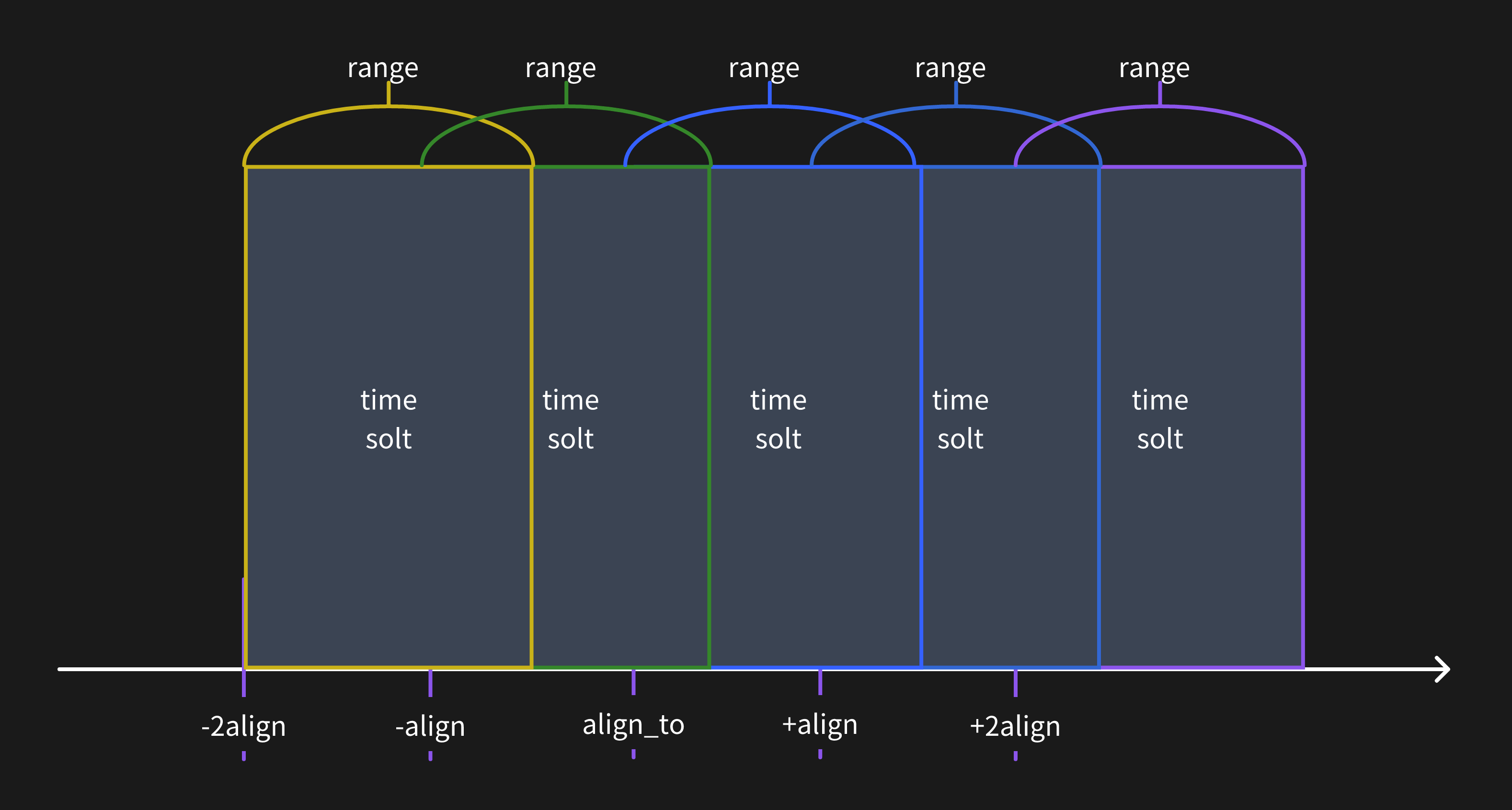
SELECT avg(temperature) RANGE '7d' from table ALIGN '1d';For each Range expression, we utilize align_to (specified by the TO keyword, the TO keyword is not specified above, which is UTC 0 time. For more usage of the TO keyword, please refer to this documentation, the align (1d) and range (7d) parameters to define time windows (each time window is called a time slot) and categorize data based on their appropriate timestamps into these time slots.
The time origin on the time axis is set at
align_to, and we segment aligned time points both forwards and backwards using align as the step size. This collection of time points is referred to asalign_ts. The formula foralign_tsis{ ts | ts = align_to + k * align, k is an integer }.For each element
tsin thealign_tsset, atime slotis defined. A time slot is a left-closed, right-open interval satisfying[ts , ts + range).
When align is greater than range, the segmented time slots are as illustrated below, and in this scenario, a single data point will belong to only one time slot.
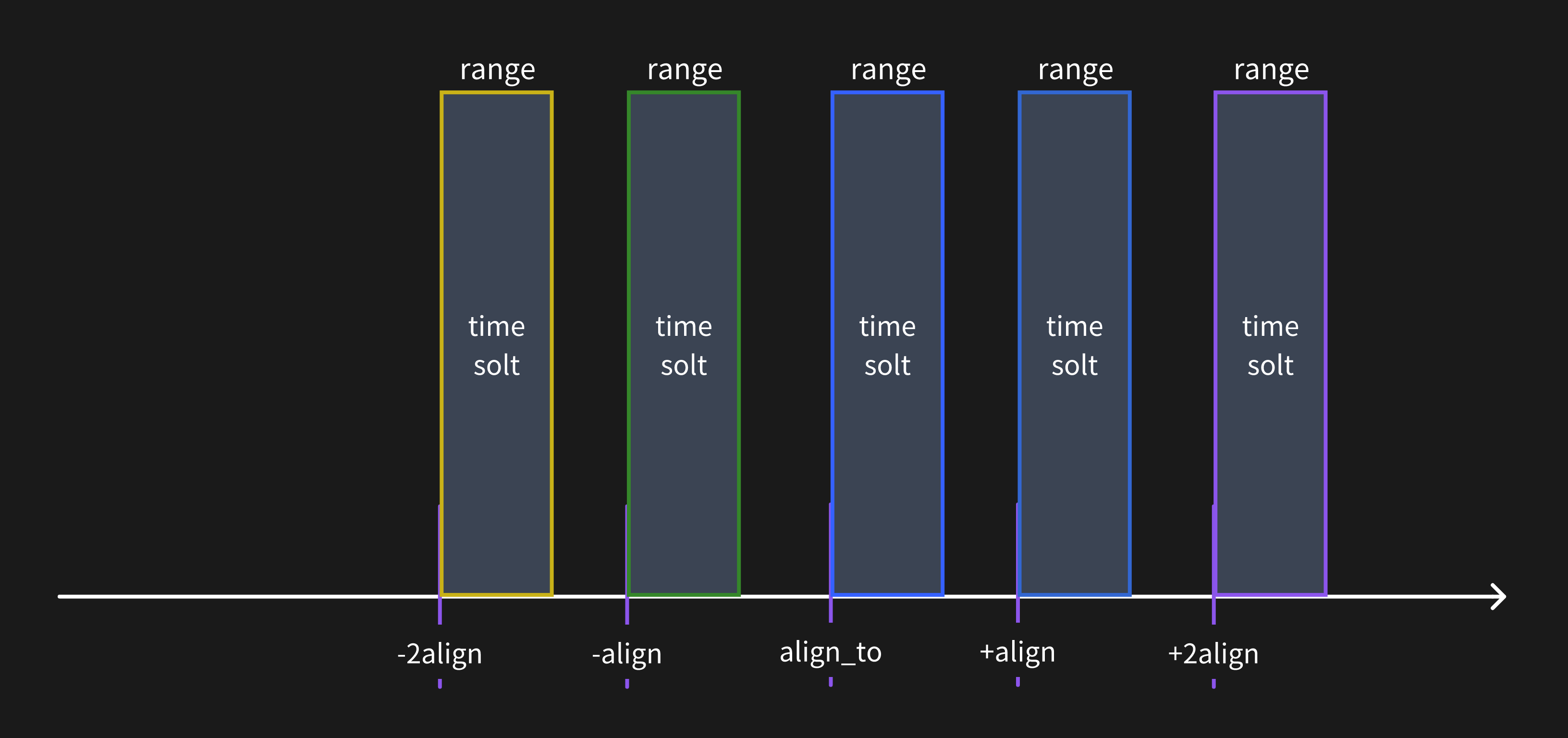
When align is smaller than range, the segmented time slots appear as shown in the following illustration. In this situation, a single data point may belong to multiple time slots.
The implementation of the Range feature utilizes the classic hash aggregation algorithm. This involves reserving a hash bucket for each time slot being sampled and placing all the data scheduled for sampling into the corresponding hash buckets.
Unlike traditional aggregation algorithms, time series data aggregation may involve overlapping data points (e.g. calculating the daily average temperature for each week). In algorithmic terms, this means a single data point may belong to multiple hash buckets, which differentiates it from the conventional hash aggregation approach.
Summary
By leveraging the SQL RANGE query syntax extension provided by GreptimeDB, combined with the powerful expressive capabilities of the SQL language itself, we can conduct more concise, elegant, and efficient analysis and querying of time series data within GreptimeDB. This approach also circumvents some of the limitations encountered in data querying with PromQL. Users can flexibly utilize RANGE queries in GreptimeDB to unlock new methods for time series data analysis and querying.


