
On this page

GreptimeDB can serve as a remote read backend for Prometheus. The last step on that path converts the columnar RecordBatch produced by the query engine into the row-oriented TimeSeries of the Prometheus protocol: group rows by their label set, and collect the samples of each series together.
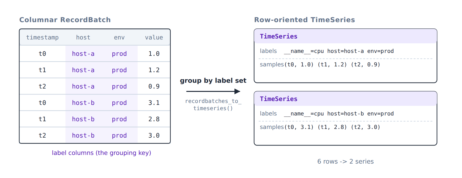
Figure 1: the columnar RecordBatch from the query engine, converted into the row-oriented TimeSeries of the Prometheus protocol
This function (recordbatches_to_timeseries) had sat untouched in the repo for a long time, until our committer @lyang24, whom we interviewed last year, opened PR #8587 and rewrote it. The PR changes exactly one file, src/servers/src/prom_store.rs.
ℹ️ Note: GreptimeDB v1.2.0-beta.1 is out and ships this optimization.
I only read this code because the PR showed up. The description includes a diagram the author drew, and its lower right corner carries a CPU profile: with 300k series and 4 concurrent reads, the RecordBatch → TimeSeries step took 36.2% of CPU, and dictionary materialization alone took 8.9%. A function that neither decompresses nor touches disk, that only moves data around in memory, burning a third of the CPU: that number is not normal.
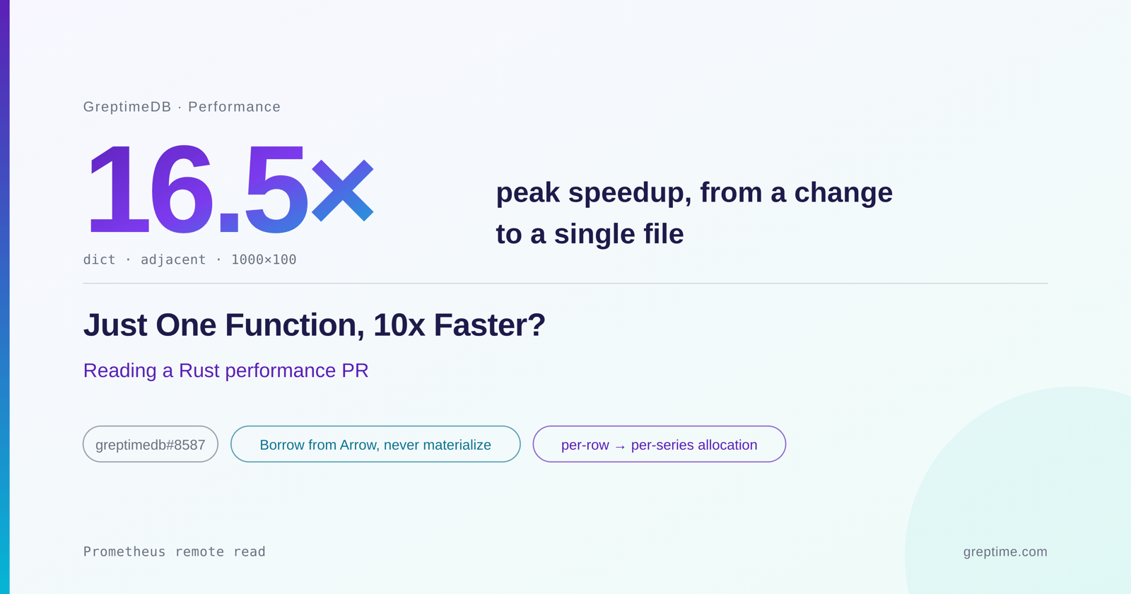
The profile came from the author, and I did not reproduce that environment. To find out how much the change itself actually gained I needed a benchmark I could run, and the bench code did not land with the PR. So I rewrote one against the public entry point and ran it on both sides of the change. The numbers before the change were not good either: 10K rows took 3.7 ms per conversion, 100K rows took 44 ms, under 3M rows per second. After the change, the best cases run more than 10x faster.
This post is my walkthrough of the PR, taking the same route as 5x Slower than Go? Optimizing Rust Protobuf Decoding Performance: write a benchmark to reproduce first, then read the code section by section. The benchmark code is in this gist.
Step 1: Reproduce the Case
First, pin down the state before the change. The bench drives the public entry point recordbatches_to_timeseries directly, through criterion:
rust
fn bench_prom_read_convert(c: &mut Criterion) {
    let mut group = c.benchmark_group("prom_read_convert");
    group.measurement_time(Duration::from_secs(5));

    // (series count, samples per series)
    let sizes = [(10, 1000), (100, 100), (1000, 100), (5000, 20)];

    for encoding in [Encoding::Dictionary, Encoding::Utf8] {
        for ordering in [Ordering::Adjacent, Ordering::Interleaved] {
            for (series, samples) in sizes {
                let rows = series * samples;
                let (schema, batch) = build_recordbatch(series, samples, ordering, encoding);

                group.throughput(Throughput::Elements(rows as u64));
                group.bench_with_input(
                    BenchmarkId::new(
                        format!("{}/{}", encoding.name(), ordering.name()),
                        format!("{series}x{samples}"),
                    ),
                    &(schema, batch),
                    |b, (schema, batch)| {
                        b.iter(|| {
                            let batches =
                                RecordBatches::try_new(schema.clone(), vec![batch.clone()])
                                    .unwrap();
                            black_box(
                                recordbatches_to_timeseries("bench_metric", batches).unwrap(),
                            )
                        });
                    },
                );
            }
        }
    }

    group.finish();
}
The three dimensions the loops iterate over come from real scenarios. For encoding, Utf8 is a plain string column, and Dictionary<UInt32, Utf8> is the label layout the PromQL read path actually returns. For ordering, adjacent means the samples of one series are contiguous in the result (query output is generally sorted by primary key, which produces this shape), and interleaved means the series alternate row by row. For size, it is series count times samples per series; a typical remote read request has few series with many points each. The labels are modeled on a real metric table: host differs for every series, while datacenter, env and job have only a handful of values.
bash
cargo bench -p servers --bench prom_read_convertThe results are as follows:
text
prom_read_convert/utf8/adjacent/100x100
                        time:   [3.6421 ms 3.6581 ms 3.6759 ms]
                        thrpt:  [2.7204 Melem/s 2.7337 Melem/s 2.7457 Melem/s]

prom_read_convert/dict/adjacent/100x100
                        time:   [4.9186 ms 4.9330 ms 4.9482 ms]
                        thrpt:  [2.0209 Melem/s 2.0272 Melem/s 2.0331 Melem/s]

prom_read_convert/dict/adjacent/1000x100
                        time:   [55.435 ms 55.574 ms 55.719 ms]
                        thrpt:  [1.7947 Melem/s 1.7994 Melem/s 1.8039 Melem/s]
The thrpt line is the throughput reported by criterion. One element here is one row, so this is around 2M rows per second.
Something else looks off besides the absolute speed: the dictionary-encoded group is 35% slower than the plain string group (2.0272M vs 2.7337M). Dictionary encoding exists to save memory and copies, so why is it slower? We will come back to this.
Step 2: What the Function Does for Every Row
Open the old code and the first step is collect_timeseries_ids. The function had carried a self-deprecating comment from the start; whoever wrote it clearly knew it was bad and just had no better place to start:
rust
/// Collect each row's timeseries id
/// This processing is ugly, hope <https://github.com/GreptimeTeam/greptimedb/issues/336> making some progress in future.
fn collect_timeseries_ids(table_name: &str, recordbatch: &RecordBatch) -> Vec<TimeSeriesId> {
It builds an owned label vector for every row:
rust
for row in 0..row_count {
    let mut labels = Vec::with_capacity(recordbatch.num_columns() - 1);
    labels.push(new_label(METRIC_NAME_LABEL.to_string(), table_name.to_string()));

    for (column_name, column_values) in columns.iter() {
        if let Some(value) = &column_values[row] {
            labels.push(new_label((*column_name).clone(), value.clone()));
        }
    }
    timeseries_ids.push(TimeSeriesId { labels });
}
And columns here is every column materialized in full, up front:
rust
.map(|(i, column_name)| {
    (column_name, recordbatch.iter_column_as_string(i).collect::<Vec<_>>())
})
The second step uses those ids as grouping keys:
rust
let mut timeseries_map: BTreeMap<&TimeSeriesId, TimeSeries> = BTreeMap::default();

for (row, timeseries_id) in timeseries_ids.iter().enumerate() {
    let timeseries = timeseries_map
        .entry(timeseries_id)
        .or_insert_with(|| TimeSeries {
            labels: timeseries_id.labels.clone(),
            ..Default::default()
        });
    // push sample
}
Because the protobuf-generated Label does not implement Eq, TimeSeriesId also needs hand-written PartialEq / Eq / Hash / Ord implementations.
The code reads clearly enough. The problem is the magnitude of the cost. Let R be the row count, S the series count, and L the average number of labels. One pass costs: R·L calls to to_string() for the full-column materialization; one Vec<Label> per row, so R heap allocations; one clone each for every label name and value, another R·L string copies; and one BTreeMap lookup per row, each on the order of log(S) comparisons. The comparison short-circuits at the first differing label, but in the worst case it has to walk the whole vector.
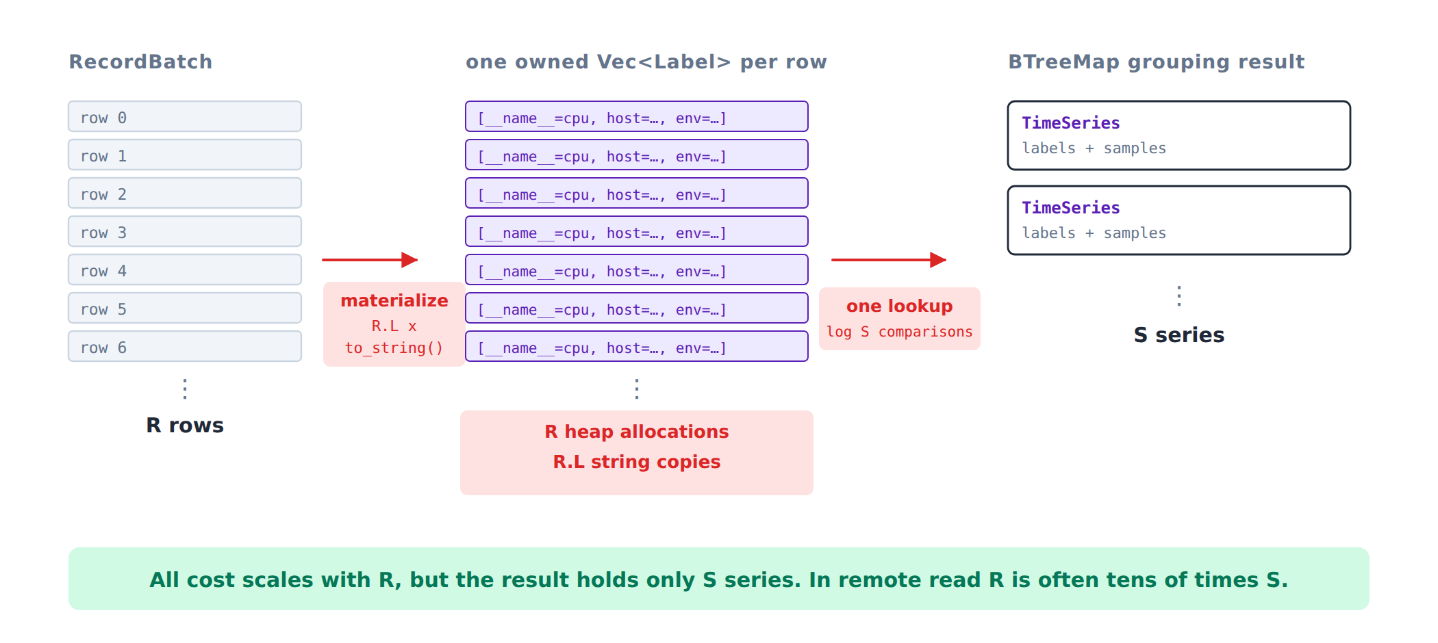
Figure 2: every cost in the old implementation scales with the row count R, and most of it goes into rebuilding the same label set over and over
So all the cost scales with the row count, while the actual information in the result is only S series. A typical remote read request pulls tens or hundreds of points per series, making R tens of times S, and most of the allocation and copying goes into rebuilding the same label set over and over.
ℹ️ Note: Both
RandShere are per-RecordBatchnumbers. Grouping happens batch by batch;recordbatches_to_timeseriesonly flattens the per-batch results, so a series that spans two batches is not merged at this step. That holds for both the old and new implementations.
Step 3: Why Dictionary Columns Were Slower
Back to the question from Step 1. The label columns returned by the PromQL read path are Dictionary<UInt32, Utf8>. Across 1000 rows, host might have only 3 distinct values, so the dictionary stores 3 strings and each row stores a u32 index. That encoding is there on purpose, kept by #8541.
But iter_column_as_string does not recognize dictionary columns. It falls back to the generic path and calls to_string() row by row. The 3 strings become 1000, every allocation upstream avoided is made again here, plus one extra dictionary lookup per row. That is where the slowdown against plain string columns comes from, and it is the 8.9% listed separately in the profile at the top of this post.
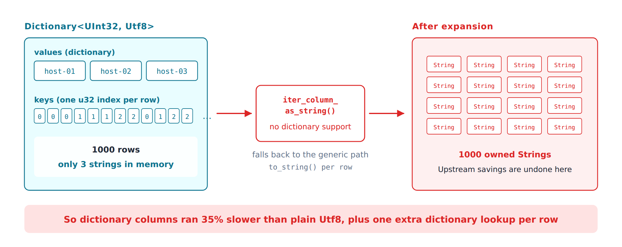
Figure 3: the dictionary encoding upstream deliberately kept, expanded by a single iter_column_as_string downstream
At this point the direction of the PR is clear: grouping only needs to read a row's value and compare it, so do not copy; borrow straight from the Arrow array. Allocate only once you have confirmed this is a series you have never seen.
Step 4: Borrow from Arrow Arrays Instead of Materializing
Copies come first. The PR wraps label columns in a borrowed view:
rust
enum LabelValues<'a> {
    Utf8(&'a StringArray),
    LargeUtf8(&'a LargeStringArray),
    Utf8View(&'a StringViewArray),
    DictionaryUtf8 {
        dictionary: &'a DictionaryArray<UInt32Type>,
        values: &'a StringArray,
    },
    Other(Vec<Option<String>>),
}

impl LabelValues<'_> {
    fn value(&self, row: usize) -> Option<&str> {
        match self {
            Self::Utf8(values) => values.is_valid(row).then(|| values.value(row)),
            Self::LargeUtf8(values) => values.is_valid(row).then(|| values.value(row)),
            Self::Utf8View(values) => values.is_valid(row).then(|| values.value(row)),
            Self::DictionaryUtf8 { dictionary, values } => dictionary
                .key(row)
                .and_then(|key| values.is_valid(key).then(|| values.value(key))),
            Self::Other(values) => values.get(row).and_then(Option::as_deref),
        }
    }
}
The four Arrow layouts a label column can actually have get one branch each: StringArray, LargeStringArray, StringViewArray, and the dictionary-encoded DictionaryArray<UInt32Type>. value(row) returns a &str borrowed from the array, with no copy and no allocation. Since LabelValues<'a> holds nothing but &'a references, the Rust compiler enforces that these &str cannot outlive the RecordBatch, rather than relying on convention.
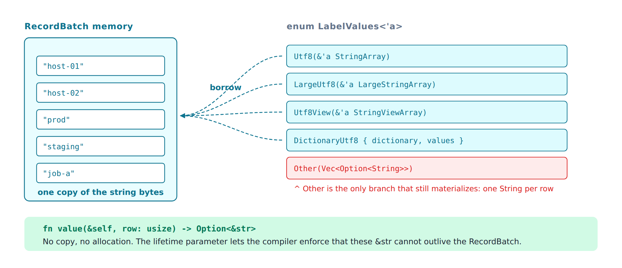
Figure 4: four Arrow layouts with one branch each, reading values by row straight from the array. Compare with Figure 3.
The dictionary branch is what Step 3 was asking for: dictionary.key(row) gets the index, and values.value(key) borrows one of the few strings in the dictionary. That is still 1000 index lookups for 1000 rows, but they all reuse the same 3 strings and never expand into 1000 owned Strings.
Label columns with a non-string type, Int32 for example, still have to be materialized and land in Other, and that path still produces one String per row. The PR also fixes what used to be a bad error path:
rust
ensure!(
    values.len() == recordbatch.num_rows(),
    error::InvalidPromRemoteReadQueryResultSnafu {
        msg: format!(
            "Cannot convert label column '{}' of datatype {:?} to string",
            column_schema.name,
            array.data_type()
        ),
    }
);
I read this differently from the PR description. The author writes that the change avoids silently omitting that column, so the old behavior was a silent skip. The code does not look that way to me. When iter_column_as_string hits a column it cannot convert into a GreptimeDB vector, it returns an empty iterator, which collects into an empty Vec. The old code then indexes column_values[row], which panics out of bounds for any non-empty batch. Nothing silent about it. Either way, an Err carrying the column name and datatype beats what was there before: when it breaks, you at least know which column.
Step 5: Grouping Without a BTreeMap
With copies handled, what remains is one tree lookup and one Vec allocation per row. The new loop looks like this. LabelColumn below is a column name plus the LabelValues from above:
rust
let columns = label_columns(&recordbatch)?;
let mut timeseries: Vec<TimeSeries> = Vec::new();
let mut timeseries_by_hash: HashMap<u64, Vec<usize>> = HashMap::new();
let mut previous_timeseries: Option<usize> = None;
for row in 0..recordbatch.num_rows() {
let timeseries_index = match previous_timeseries {
Some(index) if matches_timeseries(×eries[index].labels, &columns, row) => index,
_ => {
let hash = hash_timeseries(&columns, row);
let candidates = timeseries_by_hash.entry(hash).or_default();
match candidates
.iter()
.copied()
.find(|index| matches_timeseries(×eries[*index].labels, &columns, row))
{
Some(index) => index,
None => {
let index = timeseries.len();
timeseries.push(new_timeseries(table, &columns, row));
candidates.push(index);
index
}
}
}
};
previous_timeseries = Some(timeseries_index);
// push sample into timeseries[timeseries_index]
}The outer Some(index) if matches_timeseries(...) targets the shape of the data. Mito's SeqScan sorts by primary key and time within each PartitionRange, so the samples of one series are mostly contiguous. Comparing the current row against the series the previous row landed on is enough to reuse it on a hit, with no hash to compute. This only optimizes a common local ordering. It can break across partitions and across ranges, and correctness does not depend on it.
When the fast path breaks, and the first time each series appears, the hash path takes over. The map value is a candidate list rather than a single index, because hashes collide and a candidate still has to pass a full label comparison. Merging two different series for the sake of speed is a mistake this function cannot make.
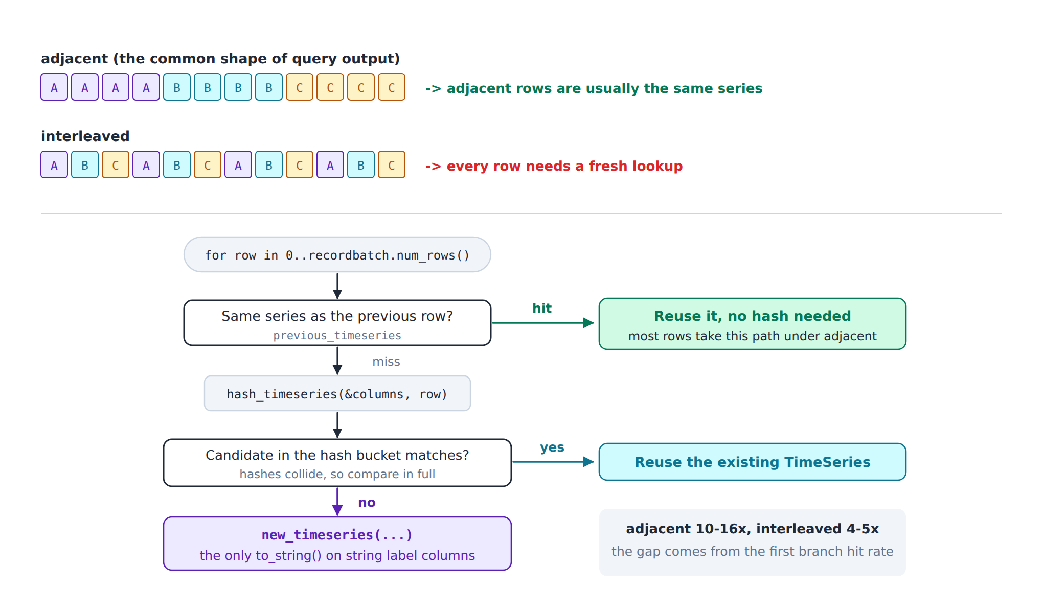
Figure 5: the three paths a row can take in the new implementation. The fast path's hit rate decides the speedup.
A row only reaches new_timeseries once it is judged to be a new series. For label columns in any of the four layouts above, the to_string() here is the only copy in the whole pass:
rust
fn new_timeseries(table: &str, columns: &[LabelColumn<'_>], row: usize) -> TimeSeries {
    let mut labels = Vec::with_capacity(columns.len() + 1);
    labels.push(new_label(METRIC_NAME_LABEL.to_string(), table.to_string()));

    for (name, value) in row_labels(columns, row) {
        labels.push(new_label(name.to_string(), value.to_string()));
    }

    TimeSeries { labels, ..Default::default() }
}
R·L copies become S·L copies (still counted within one batch). The whole optimization moves allocation from "every iteration" to "the iteration that finds something new".
Step 6: Do Not Change the Observable Behavior
This is protocol-layer code, so a change should touch externally observable behavior as little as possible and avoid leaving compatibility problems downstream. Three parts of the PR are there for exactly that.
The old implementation used a BTreeMap, so output was label-ordered for free. The new one uses a Vec, ordered by first appearance. So a sort was added at the end, with the comparison copied from the old Ord for TimeSeriesId:
rust
timeseries.sort_unstable_by(|left, right| compare_timeseries_labels(&left.labels, &right.labels));One S·log(S) sort is negligible against what was saved.
NULL semantics have to match too. The old code used if let Some(value) to skip NULL labels, meaning the label simply does not exist. The new code uses filter_map to keep that behavior, and dictionary columns add one more case: the key is NULL, or the value the key points to is NULL. That is where the two layers of and_then above come from.
Since NULL labels are skipped, one series' label sequence can be a prefix of another's, so the comparison has to be careful:
rust
fn matches_timeseries(labels: &[Label], columns: &[LabelColumn<'_>], row: usize) -> bool {
    let mut labels = labels.iter().skip(1);
    for (name, value) in row_labels(columns, row) {
        let Some(label) = labels.next() else {
            return false;
        };
        if label.name != name || label.value != value {
            return false;
        }
    }

    labels.next().is_none()
}
The final labels.next().is_none() is what handles that; without it, {host=a} and {host=a, env=prod} would be treated as the same series. The skip(1) at the start skips the special __name__ label, which is determined by the table name and is identical across a RecordBatch, so there is nothing to compare.
Results
Measured on an Apple M4 Max running macOS. "before" is the old implementation, "after" is the merged 32a6fc0915; the two differ only in prom_store.rs. Criterion ran 100 samples per case, and every case reports p = 0.00 < 0.05.
Dictionary-encoded labels (Dictionary<UInt32, Utf8>, the real layout on the PromQL read path):
| Ordering | Series × samples | Before | After | Speedup | Change |
|---|---|---|---|---|---|
| adjacent | 10×1000 | 4.29 ms | 292 µs | 14.7× | −93.2% |
| adjacent | 100×100 | 4.93 ms | 335 µs | 14.7× | −93.2% |
| adjacent | 1000×100 | 55.6 ms | 3.38 ms | 16.5× | −93.9% |
| adjacent | 5000×20 | 61.8 ms | 4.98 ms | 12.4× | −91.9% |
| interleaved | 10×1000 | 4.31 ms | 820 µs | 5.3× | −81.0% |
| interleaved | 100×100 | 4.67 ms | 870 µs | 5.4× | −81.3% |
| interleaved | 1000×100 | 49.7 ms | 9.03 ms | 5.5× | −81.8% |
| interleaved | 5000×20 | 54.1 ms | 10.4 ms | 5.2× | −80.8% |
Plain Utf8 labels:
| Ordering | Series × samples | Before | After | Speedup | Change |
|---|---|---|---|---|---|
| adjacent | 10×1000 | 3.08 ms | 288 µs | 10.7× | −90.8% |
| adjacent | 100×100 | 3.66 ms | 319 µs | 11.5× | −91.3% |
| adjacent | 1000×100 | 43.6 ms | 3.19 ms | 13.7× | −92.7% |
| adjacent | 5000×20 | 49.8 ms | 4.65 ms | 10.7× | −90.7% |
| interleaved | 10×1000 | 3.12 ms | 770 µs | 4.1× | −75.4% |
| interleaved | 100×100 | 3.44 ms | 832 µs | 4.1× | −75.6% |
| interleaved | 1000×100 | 37.9 ms | 8.46 ms | 4.5× | −77.7% |
| interleaved | 5000×20 | 42.3 ms | 10.1 ms | 4.2× | −76.2% |
Throughput went from 1.8M–3.2M rows per second to 9.6M–34.8M, and no case got slower.
The adjacent groups are much faster, 10–16x, and that comes from the fast path in Step 5: only the first row of each series needs a hash, roughly S/R of them. The interleaved groups compute a hash, look it up and compare on every row, and still land at 4–5x. Real query results mostly have the adjacent shape.
Dictionary columns improved the most because they had the most extra cost to begin with. At adjacent/1000×100 a dictionary column went from 55.6 ms to 3.38 ms, roughly level with the 3.19 ms of a plain string column, and the "dictionary is slower than plain strings" anomaly from Step 1 is gone.
Summary
The data structures did change: a BTreeMap became a Vec plus a hash index, a previous-series fast path was added, and the ordered output became one sort at the end. But most of the gain does not come from any of that. It comes from two plain things: do not copy what you can borrow, and do not repeat per row what you can do once.
hash_timeseries currently uses DefaultHasher, which on this toolchain is SipHash-1-3 with a fixed key, and the algorithm itself is not covered by the stable API guarantee. Swapping in something like ahash would be a reasonable performance experiment. The full sort at the end exists only to preserve the ordering of the previous BTreeMap; if we can confirm nothing downstream depends on it, that can go too.
The dictionary-column trap from Step 3 is the part worth remembering. Upstream deliberately kept the dictionary encoding to save memory, and one iter_column_as_string downstream expanded it anyway, into something slower than not using a dictionary at all. This is hard to find without a benchmark.
Reproduce It Yourself
The bench code is in this gist. The PR touches one file, so the comparison does not need a full rebuild of the repo:
bash
# 0) Put the bench file in src/servers/benches/, and append to src/servers/Cargo.toml:
#    [[bench]]
#    name = "prom_read_convert"
#    harness = false

# 1) Create a temporary worktree on the parent commit of the change
git worktree add /tmp/gdb-8587-before a0e6f0b4
cp src/servers/benches/prom_read_convert.rs /tmp/gdb-8587-before/src/servers/benches/

# 2) Run the before baseline
cd /tmp/gdb-8587-before
cargo bench -p servers --bench prom_read_convert -- \
    --warm-up-time 2 --measurement-time 4 --save-baseline before

# 3) Back to the code with the PR, run after; criterion reports change% automatically
cd -
cargo bench -p servers --bench prom_read_convert -- \
    --warm-up-time 2 --measurement-time 4 --baseline before
The numbers in this post came from a single worktree: run before first, then swap prom_store.rs for the 32a6fc0915 version, rebuild and run after, sharing one criterion data directory.
References
- The PR this post walks through, contributed by @lyang24: greptimedb#8587 perf(servers): optimize PromQL read conversion
- Benchmark code and full data: gist: prom_read_convert.rs
- The optimized source:
src/servers/src/prom_store.rs - The upstream PR that kept the dictionary encoding: #8541
- The issue the old comment pointed at for years: #336
- The previous performance post: 5x Slower than Go? Optimizing Rust Protobuf Decoding Performance
- Our interview with the PR author: GreptimeDB Committer Interview: @lyang24
- The release that ships this optimization: GreptimeDB v1.2.0-beta.1
- Prometheus remote read API: https://prometheus.io/docs/prometheus/latest/querying/remote_read_api/
- Arrow array types:
StringArray,StringViewArray,DictionaryArray - criterion.rs book: https://bheisler.github.io/criterion.rs/book/index.html


