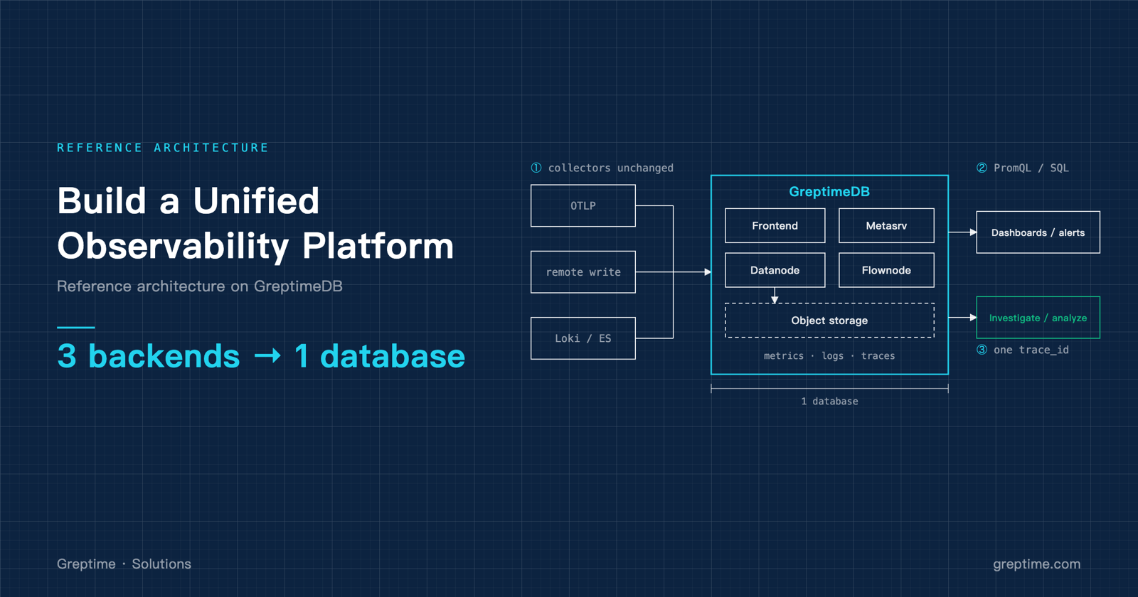
This article assumes you have already decided to put metrics, logs, and traces into one database. Why unify, and why now, is covered in our earlier post on the history of observability unification. This one covers what comes after that decision: which components to deploy, how data flows, which decisions are still yours to make, and what the topology looks like at three scales: standalone, small cluster, and large cluster. The architecture fits in one sentence: leave the collectors alone and point them at one GreptimeDB; dashboards and alerts go through PromQL, incident investigation and long-range analysis through SQL.

The validation environment is the official OpenTelemetry Astronomy Shop demo: 14 services, SDKs in several languages, and a default backend of Jaeger, OpenSearch, and Prometheus. We replaced those three with a single GreptimeDB v1.2.0 standalone instance, plus a node_exporter and a Prometheus that only scrapes. The configuration, table schemas, query results, and incident records in this article come from that environment; the complete setup is in the greptimedb-observability-playground repository. Enterprise-only features are marked where they come up.

Three workloads the platform has to carry

Dashboards and alerts. Grafana panels refresh every few seconds and alert rules evaluate every minute, over the last few minutes to few hours of data. Many queries, each small, each latency-sensitive.

Incident investigation. One investigation moves between metrics, logs, and traces: from an alert to the slow service, from the service to the slow call chain, from the call chain to the error logs and node resources of that time window. The queries are exploratory; nobody knows in advance how many there will be, and humans are no longer the only ones issuing them. In our Agent RCA Bench, one agent investigation averaged thirty to forty tool calls, with some approaching fifty.

Long-range analysis. Capacity planning, weekly reports, cost attribution: scans over weeks or months of data, heavy per query, infrequent.

The usual setup gives the first two workloads to a monitoring stack (Prometheus + Loki + Tempo, or Elasticsearch) and copies data into an analytical database for the third. This architecture runs all three on the same data and the same system. It does not cover APM front ends, on-call scheduling, or parsing rules at the collection edge; those stay with whatever you use today.

Reference architecture

Collectors keep their existing protocols and write to one GreptimeDB; two classes of query workload sit on top.

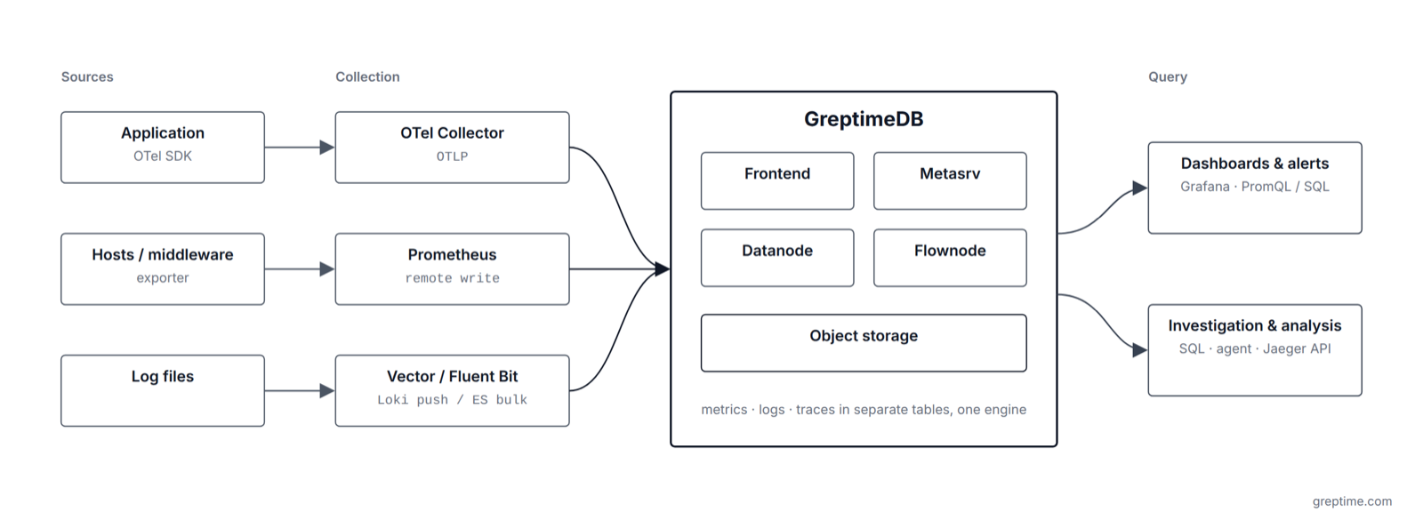
On the write side, every signal keeps the protocol it already speaks, and the collectors stay as they are. GreptimeDB exposes one write endpoint per protocol:

Signal	Protocol	Endpoint	Where it lands
metrics	Prometheus remote write	/v1/prometheus/write	Metric Engine: one logical table per metric, all sharing a physical table
metrics / logs / traces	OTLP/HTTP	/v1/otlp/v1/{metrics,logs,traces}	metrics: one table per metric; logs: opentelemetry_logs by default; traces: opentelemetry_traces by default
logs	Loki Push API	/v1/loki/api/v1/push	tables created from labels; an optional pipeline parses the line
logs	Elasticsearch _bulk	/v1/elasticsearch/_bulk	index maps to table
logs / metrics	Vector greptimedb_logs / greptimedb_metrics sink	HTTP 4000 / gRPC 4001	table per sink configuration
logs / metrics / traces	Fluent Bit HTTP or OpenTelemetry output	/v1/ingest, /v1/otlp/v1/*, /v1/prometheus/write	table per output configuration

An OTLP exporter appends the signal path itself, so the Collector endpoint is written as /v1/otlp; raw HTTP clients post to the full path.

The query side has three entry points: SQL (MySQL on 4002, PostgreSQL on 4003, HTTP on 4000), the PromQL HTTP API (/v1/prometheus/api/v1/query and query_range), and the Jaeger-compatible API (/v1/jaeger). Grafana connects through the GreptimeDB data source plugin, the Prometheus data source, or the MySQL data source; all three can coexist.

After 2 hours 16 minutes of the demo running on a laptop, the database held 860 tables:

• opentelemetry_traces, opentelemetry_logs, and two trace auxiliary tables, from OTLP;
• 375 application and container metric tables (http_server_request_duration_seconds_bucket, container_memory_usage_total_bytes, jvm_*, dotnet_*, and so on), from OTLP metrics;
• 264 node_* and 217 greptime_* tables from node_exporter and GreptimeDB's own /metrics, scraped by Prometheus and written through remote write.

Total disk: 154 MB.

Decisions you have to make

Collector

Three options: an OTel Collector for all three signals; keep the existing Prometheus or Alloy for metrics and add Vector or Fluent Bit for logs; or have application SDKs write to GreptimeDB directly.

We recommend the OTel Collector as the main collector, with one exporter per signal pointing at the same /v1/otlp endpoint and the traces exporter carrying the x-greptime-pipeline-name: greptime_trace_v1 header. When all three signals leave the same Collector, the resource attributes (service.name, k8s.pod.name, and the rest) are consistent across the three tables, and cross-signal correlation depends on those fields. If you already scrape with Prometheus, point remote write at GreptimeDB and leave the exporters alone. Vector has no traces sink, so use it for logs only.

The Collector configuration in the demo:

exporters:
  otlphttp/traces:
    endpoint: http://greptimedb:4000/v1/otlp
    headers:
      x-greptime-pipeline-name: greptime_trace_v1
      x-greptime-hints: ttl=7d
  otlphttp/logs:
    endpoint: http://greptimedb:4000/v1/otlp
  otlphttp/metrics:
    endpoint: http://greptimedb:4000/v1/otlp

The three exporters are separate because GreptimeDB uses request headers to decide how each signal is processed (the pipeline for traces, the table name and pipeline for logs), and a single exporter cannot set them independently. x-greptime-hints: ttl=7d gives the trace table a 7-day TTL at creation.

Each metric should take only one path. The demo's base Collector configuration includes the host_metrics and prometheus/ad receivers (the ad service exposes a Prometheus-format /metrics). We removed both and let Prometheus scrape host and ad metrics and remote-write them, because a Prometheus-format metric that arrives through both OTLP and remote write fails on write with a timestamp type conflict.

How to split tables

Each signal gets its own tables. GreptimeDB applies the same column semantics (Tag, Timestamp, Field) and the same columnar engine to all three, but schema, indexes, TTL, and the append-only setting are per table.

Our recommendation: split tables by signal, partition by volume.

• Metrics go through the Metric Engine. Prometheus remote write creates logical tables automatically, and many logical tables share one physical wide table, which compresses better and ingests faster than one table per metric.
• Logs use append-only tables, with indexes chosen by query pattern: an inverted index for columns filtered by equality, a skipping index for high-cardinality point-lookup columns such as trace_id, and a full-text index for body when keyword search is needed. Text logs are parsed into columns by a pipeline at write time, so queries do not parse on the fly.
• Traces use the default schema of the greptime_trace_v1 pipeline: one row per span, service_name as a Tag, attributes flattened into columns automatically.
• Wide events (one wide record per request, tens to hundreds of fields) get their own table, with a primary key and indexes designed for that shape.

The three main tables in the demo:

Table	Source	Columns	Rows	Disk
opentelemetry_traces	OTLP traces, greptime_trace_v1	193	867,803	98 MB
opentelemetry_logs	OTLP logs	14	249,098	30 MB
greptime_physical_table	Prometheus remote write, shared by 481 logical tables	163	4,307,330	23 MB

The 193 columns of the traces table come from attribute flattening; column names such as resource_attributes.service.namespace and span_attributes.http.request.body.size come from there, and the table grows one column for every distinct attribute the 14 services emit. The logs table keeps the 14 default OTLP columns, with resource attributes in the resource_attributes JSON column; queries read the service name with json_get_string(resource_attributes, '["service.name"]'). SHOW CREATE TABLE node_cpu_seconds_total shows ENGINE=metric and on_physical_table = 'greptime_physical_table': the 264 node_* and 217 greptime_* logical tables all live on that physical table.

Flattening into columns and keeping JSON each cost something. Flattened columns can be indexed and filtered directly; the cost is a schema that grows with the attributes, and type differences between SDKs surface at write time. In the demo, the quote service is PHP, and its SDK writes http.request.body.size as a string, with an empty string when the length is unknown. Other SDKs write an integer, GreptimeDB had created an integer column, and when the empty string arrived the whole span was rejected; the Collector log showed Partial success response and dropped_spans. The fix is a transform processor in the Collector that converts numeric strings to integers and drops the empty ones. Keeping attributes in JSON gives a stable schema; the cost is parsing JSON on every attribute access. GreptimeDB v1.2.0 introduced the JSON2 type, and we will ship a v2 trace pipeline built on it to reduce the cost of parsing JSON.

The rule for tables versus partitions: data that differs logically (different schema, different retention) goes into different tables; a table is partitioned only when a single node can no longer carry it. One thing that is easy to miss in cluster mode: the Metric Engine's default physical table has one partition, so all remote write lands on the same datanode. Either create a partitioned physical table on a label such as namespace before writing, or repartition at runtime.

Isolating the hot path

Dashboards and alerts are the most latency-sensitive workload in this system; a single heavy investigation or analysis query scans far more data. When both share one system, isolate them at two levels.

Once the raw tables get large enough, dashboards and alerts move to a Flow sink table; investigation and analysis keep scanning the raw tables.

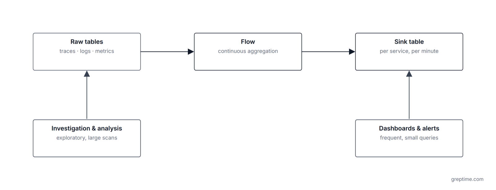
At the data level, Flow is a materialized view: a fixed aggregate kept current as data arrives. The judgement is the same as for any materialized view. The query has to be fixed and repeated — a dashboard panel, an alert rule — plus at least one of: the raw scan behind it has become expensive; the raw data is on a short TTL and the aggregate has to outlive it; or the number is not in the raw table at all and has to be derived from it, such as a per-service error rate computed from spans. None of these bind at small scale: dashboards on the Metric Engine are already fast, and the demo's two hours of traces are 860,000 rows in 98 MB. The Flow below is the last two cases at once — it derives a metric from spans, and it survives the 7-day TTL on the trace table.

Flow computes the aggregate at a fixed interval and writes it to a sink table; dashboards and alerts then read the sink table, and only investigation and analysis scan the raw tables. In the Poizon case, Flow maintains 10-second, 1-minute, and 10-minute rollups, and P99 dashboard query latency dropped from seconds to milliseconds. Alert rules work the same way: compute each service's per-minute error count in Flow, and the Grafana alert only compares against a small table. The Flow in the demo:

CREATE FLOW IF NOT EXISTS service_error_rate_1m
SINK TO service_error_rate_1m
EVAL INTERVAL '30s'
AS
SELECT
  service_name,
  date_bin('1 minute'::INTERVAL, "timestamp") AS time_window,
  count(*) AS total,
  sum(CASE WHEN span_status_code = 'STATUS_CODE_ERROR' THEN 1 ELSE 0 END) AS errors
FROM opentelemetry_traces
WHERE span_kind = 'SPAN_KIND_SERVER'
  AND "resource_attributes.service.namespace" = 'opentelemetry-demo'
GROUP BY service_name, time_window;

Flow creates the sink table itself, with service_name as the primary key and time_window as the time index. Two hours of data is 2,485 rows and 60 KB in the sink table, against 860,000 rows in the raw traces table. The rows for checkout and payment across six one-minute windows around an incident (the incident itself is covered below):

SELECT service_name, time_window, total, errors
FROM service_error_rate_1m
WHERE service_name IN ('checkout', 'payment')
  AND time_window BETWEEN '2026-09-15 14:42:00' AND '2026-09-15 14:47:00'
ORDER BY time_window, service_name;

service_name	time_window	total	errors
checkout	14:42	2	0
payment	14:42	2	0
checkout	14:43	7	5
payment	14:43	7	5
checkout	14:44	2	2
payment	14:44	2	2
checkout	14:45	4	2
payment	14:45	3	2
checkout	14:46	1	0
payment	14:46	1	0
checkout	14:47	1	0
payment	14:47	2	0

Alert rules run windowed queries against this table and scan a few thousand rows each time.

At the node level, use frontend groups. A GreptimeDB cluster can run several groups of frontends; the Helm chart lets you give read and write groups their own replica counts and resource limits, and dashboards, alerts, and collectors point at different services. This level isolates query planning and protocol handling; the datanodes are still shared. Isolating heavy scans at the storage level requires Read Replicas (read-only datanodes) or Datanode groups, both Enterprise features. Contact us for a demo.

Retention and storage

Object storage is the default in this architecture. GreptimeDB's on-disk data is roughly 1/8 to 1/10 of the raw input, long-range analysis needs months of retention, object storage is cheaper than local disk, and scaling out does not copy data files between datanodes. Local disk only holds the query cache and the WAL; start at 200 GB and adjust for your disk, cache configuration, and WAL retention.

TTL is set per table, and a table-level setting overrides the database-level one. A reasonable starting point: metrics and Flow sink tables for 90 days or more, traces for 7 to 14 days, raw logs according to compliance requirements, wide events according to volume. Adjust these to your query habits; the sink table should outlive the raw table, because long-range analysis mostly reads aggregates.

There are two WAL modes, Local and Remote. Local WAL uses the raft-engine embedded in the datanode and needs no extra component; a datanode replays the WAL on restart, and recovery time depends on how much data has to be replayed (the memtable data not yet flushed to persistent storage). Remote WAL uses Kafka; when a datanode fails, Metasrv can move its regions to other nodes directly, so recovery is fast, at the cost of running a Kafka. Use Local WAL for standalone and small clusters, and Remote WAL for clusters with high-availability requirements.

Who uses which query interface

The three query entry points serve three kinds of users.

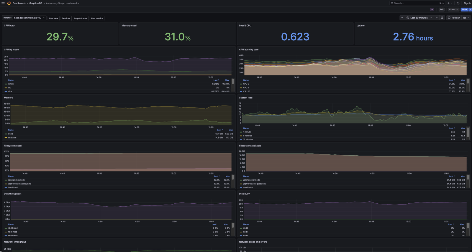
PromQL serves DevOps and existing Grafana dashboards. GreptimeDB's PromQL HTTP API is Prometheus-compatible: point an existing dashboard at GreptimeDB and it works, and alert rules are evaluated by Grafana's native alerting. The demo's host dashboard is entirely standard expressions on the Prometheus data source; expressions such as 1 - avg(rate(node_cpu_seconds_total{job="node",mode="idle"}[5m])) are the same as in community Grafana dashboards, and nothing changed when the data source was switched to GreptimeDB.

Host dashboard: node_exporter → Prometheus scrape → remote write into GreptimeDB, Prometheus data source.

SQL serves investigation, analysis, and agents. Grafana's GreptimeDB data source plugin offers SQL queries plus Logs and Traces query types with OpenTelemetry column-mapping presets. Notebooks, BI tools, and agents connect over the MySQL or PostgreSQL protocol. We also provide the GreptimeDB MCP Server, which lets an LLM talk to GreptimeDB directly.

The Jaeger-compatible API serves existing trace tools: /v1/jaeger exposes /api/services, /api/traces, and /api/traces/{trace_id}. Grafana's Jaeger data source can point at it directly, or you can keep using the Jaeger UI.

What an investigation looks like in one database

With one query surface, cross-signal correlation is a handful of queries on the same trace_id. Both examples below come from the demo's actual data.

The demo ships with fault switches. With paymentFailure set to 100%, checkout requests return HTTP 422. The errors in the 14:43 to 14:45 windows of the sink table above are this incident, and the error-rate curve on the Overview dashboard spikes for those three minutes. To get from the sink table back to the raw table, first pull the failed server-side spans:

SELECT "timestamp", service_name, span_name, duration_nano / 1e6 AS ms, trace_id
FROM opentelemetry_traces
WHERE span_kind = 'SPAN_KIND_SERVER'
  AND span_status_code = 'STATUS_CODE_ERROR'
  AND service_name IN ('checkout', 'payment')
ORDER BY "timestamp" DESC
LIMIT 6;

timestamp	service_name	span_name	ms	trace_id
14:45:29.778	payment	oteldemo.PaymentService/Charge	0.5	292a59a2…
14:45:25.556	checkout	oteldemo.CheckoutService/PlaceOrder	4242.7	292a59a2…
14:45:08.962	payment	oteldemo.PaymentService/Charge	0.5	8f17e37c…
14:45:05.719	checkout	oteldemo.CheckoutService/PlaceOrder	3374.1	8f17e37c…
14:44:13.247	payment	oteldemo.PaymentService/Charge	0.4	de318fc3…
14:44:09.866	checkout	oteldemo.CheckoutService/PlaceOrder	3454.4	de318fc3…

Each pair of error spans shares a trace_id. Take the first one and query the whole call chain, CLIENT and SERVER spans only:

service	span	kind	ms	status
frontend-proxy	POST	SERVER	4396.8	UNSET
frontend	POST /api/checkout	SERVER	4396.8	UNSET
checkout	oteldemo.CheckoutService/PlaceOrder	SERVER	4242.7	ERROR
checkout	oteldemo.PaymentService/Charge	CLIENT	48.4	ERROR
payment	oteldemo.PaymentService/Charge	SERVER	0.5	ERROR

The span_status_message on checkout: failed to charge card: could not charge the card: rpc error: code = Unknown desc = Payment request failed. Invalid token.. The same trace_id against opentelemetry_logs returns a few dozen log records for this call chain. The ones that matter for the failure:

SELECT "timestamp", json_get_string(resource_attributes, '["service.name"]') AS service, severity_text, body
FROM opentelemetry_logs
WHERE trace_id = '292a59a2b413877ef2392a28d1e52c87'
ORDER BY "timestamp";

timestamp	service	severity	body
14:45:25.421	frontend-proxy		"POST /api/checkout HTTP/1.1" 422 … 4396 4396
14:45:25.651	checkout	INFO	[PlaceOrder]
14:45:29.307	shipping	INFO	Requesting quote
14:45:29.778	payment	info	Charge request received.
14:45:29.778	payment	warn	Payment request failed. Invalid token. demo.user_context.loyalty_level=gold
14:45:29.817	frontend	info	Checkout payment declined

The payment service logs this at warn level while the corresponding span is ERROR; each level is chosen by that service's own code.

Logs & traces: waterfall, span details, and correlated logs by Trace ID.

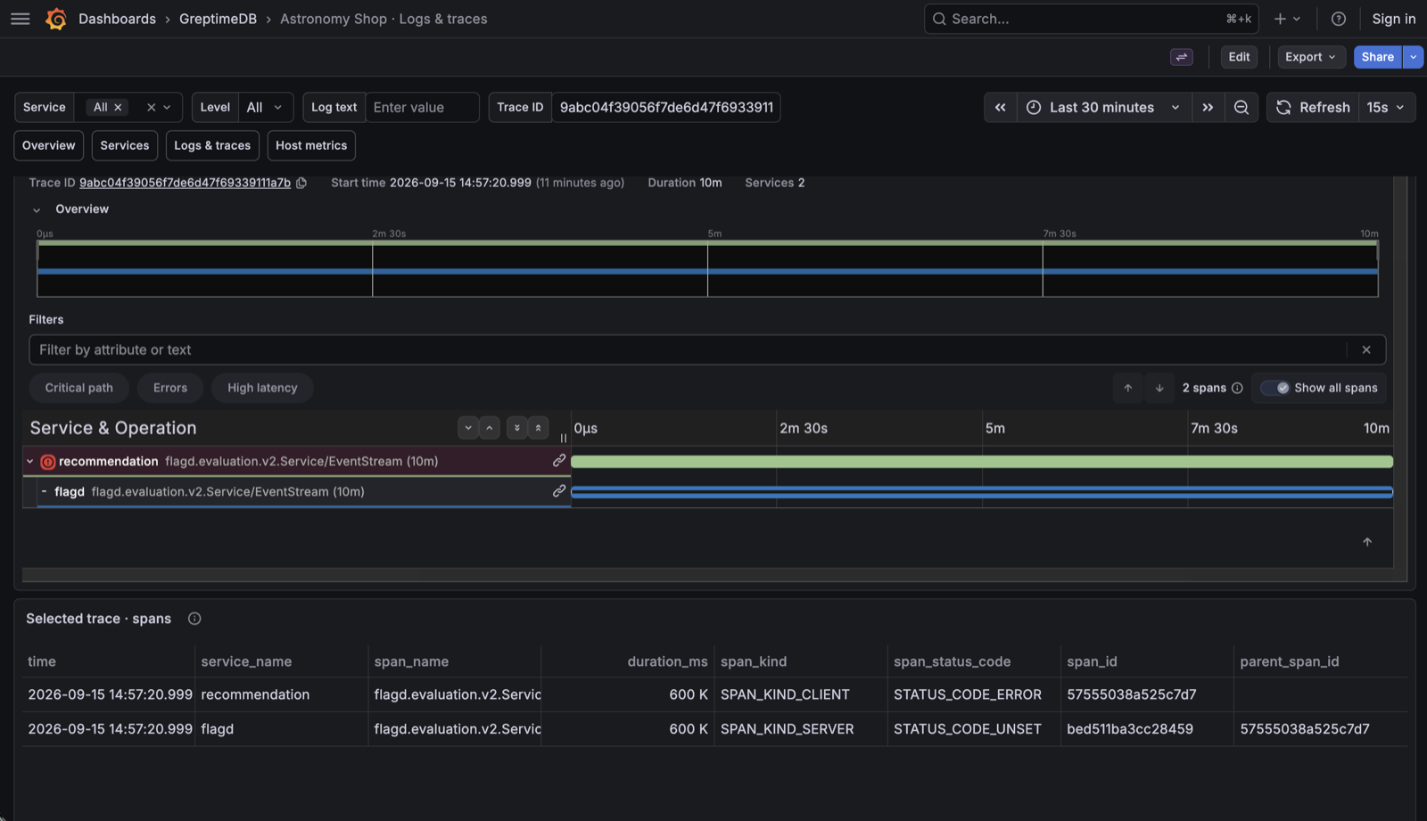
Latency questions are a self-join. Every row in opentelemetry_traces is one span, and the client span and server span of one call are linked through trace_id and parent_span_id, so one join puts both durations on the same row:

SELECT
  c.trace_id,
  c.service_name        AS client,
  s.service_name        AS server,
  s.span_name,
  c.duration_nano / 1e6 AS client_ms,
  s.duration_nano / 1e6 AS server_ms
FROM opentelemetry_traces c
JOIN opentelemetry_traces s
  ON s.trace_id = c.trace_id
 AND s.parent_span_id = c.span_id
WHERE c.span_kind = 'SPAN_KIND_CLIENT'
  AND s.span_kind = 'SPAN_KIND_SERVER'
  AND c."timestamp" > now() - INTERVAL '30 minutes'
ORDER BY client_ms DESC
LIMIT 30;

Take a 10-second checkout request from the demo, trace 8ea79526…. Restricted to that trace_id, the entry call and the pairs where checkout is the caller:

client	server	span_name	client_ms	server_ms
frontend	checkout	oteldemo.CheckoutService/PlaceOrder	9315.9	9226.3
checkout	product-catalog	oteldemo.ProductCatalogService/GetProduct	1650.1	1161.0
checkout	product-catalog	oteldemo.ProductCatalogService/GetProduct	1181.0	768.2
checkout	product-catalog	oteldemo.ProductCatalogService/GetProduct	815.5	452.5
checkout	product-catalog	oteldemo.ProductCatalogService/GetProduct	627.5	272.6
checkout	shipping	POST /get-quote	490.9	4.3
checkout	currency	oteldemo.CurrencyService/Convert	423.0	0.02
checkout	currency	oteldemo.CurrencyService/Convert	372.5	0.03
checkout	payment	oteldemo.PaymentService/Charge	339.7	0.57
checkout	currency	oteldemo.CurrencyService/Convert	304.0	0.03
checkout	shipping	POST /ship-order	251.3	0.72
checkout	currency	oteldemo.CurrencyService/Convert	219.0	0.03
checkout	cart	POST /oteldemo.CartService/GetCart	202.7	5.53
checkout	email	POST /send_order_confirmation	186.8	18.36
checkout	currency	oteldemo.CurrencyService/Convert	121.9	0.03

For GetProduct, client and server durations are in the same range. For Convert, Charge, and get-quote, server-side processing is under 1 ms while the client waits 120 to 490 ms; the difference sits on the call path between checkout and those services. The cause has to be found at the application or network level; this table tells you where the gap is.

Agent RCA Bench measured how the query interface affects agent-driven investigations. Six models, 14 incidents, two repetitions each, 168 end-to-end investigations per interface, over the native Prometheus, Loki, and Tempo APIs and read-only SQL plus PromQL on GreptimeDB. With the same models, prompts, and raw data, the GreptimeDB interface produced 130 correct diagnoses against 105 for the three-backend interface, read 48% fewer input tokens, and cost about 45% less at model API prices. All six models read fewer tokens on the GreptimeDB interface, and five of the six were more accurate. The comparison swaps the whole interface bundle at once, storage, query language, and tool design together, so the storage engine's contribution is not isolated. On the GreptimeDB interface, only three investigations used a cross-signal JOIN; the models mostly did within-table pairing like the example above, plus comparisons across time windows. The full protocol, per-run records, and the scope of each claim are in the report.

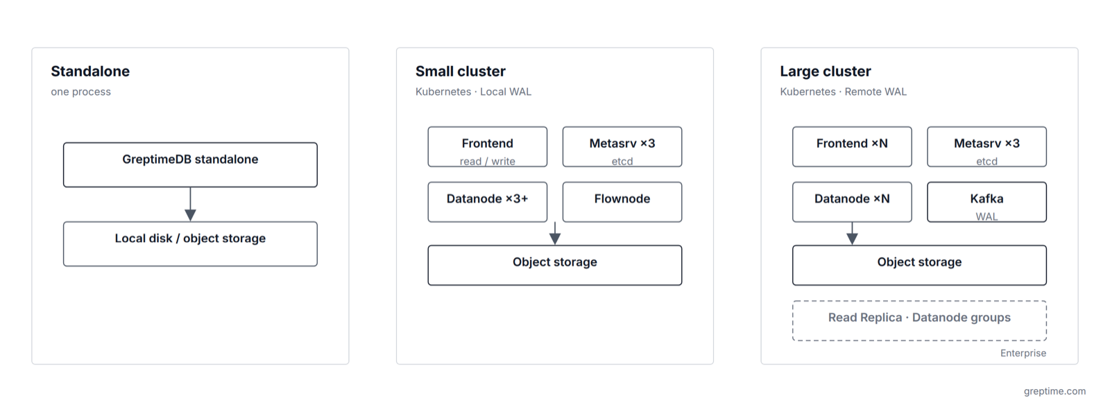
Three scale tiers

Standalone, small cluster, and large cluster topologies.

Standalone

One GreptimeDB process provides everything, as a container or a binary, with data on local disk or object storage. This fits one team, one Kubernetes namespace, or a staging environment. The demo runs at this tier.

Our suggested starting point is 8 cores, 32 GB of memory, and 200 GB of local disk, which corresponds to roughly 300,000 data points per second of ingestion and 200 QPS of simple queries. Whether you get there depends on schema, row width, indexes, and query time ranges, so validate with your own workload. Keep CPU to memory at 1:4; ingestion takes about 30% of the CPU.

This tier usually does not need Flow. Add it when dashboard queries slow down; the definitions are the same on standalone and on a cluster, so nothing has to be rewritten later.

Small cluster

Deploy on Kubernetes with the GreptimeDB Operator and Helm chart. The components are Metasrv, Frontend, Datanode, and Flownode; metadata lives in etcd or MySQL / PostgreSQL, data files in object storage. The starting production shape is three replicas each of Metasrv and etcd, Frontend split into read and write groups, three or more Datanodes, one Flownode, and Local WAL.

Two things this tier needs that standalone does not: The Metric Engine physical table must be partitioned by label, otherwise all remote write goes to one datanode. Large tables (logs, traces, wide events) are partitioned on a high-selectivity column such as service_name or namespace; opentelemetry_traces already partitions on trace_id, 16 partitions by default. The Collector configuration, remote write address, Flow definitions, and Grafana dashboards carry over from standalone unchanged. Without Remote WAL, this cluster's availability still depends on Kubernetes rescheduling pods, so mount local disks through PVCs.

Large cluster

When ingestion and query concurrency go up another order of magnitude, three things change. We recommend switching to Remote WAL, so that when a datanode fails its regions move to other nodes without a local replay. Datanodes scale out with the number of partitions and Frontends with query concurrency, independently. Object storage capacity stops being a design constraint: in the OceanBase Cloud case, 80-plus clusters keep 7 days and 300 TB of logs and SQL audit data at about 1 GB/s of writes.

Changing indexes, repartitioning, and migrating regions all run at runtime in the open-source edition, as manual operations.

Beyond open source, there are: read-only datanodes (Read Replicas) move analytical scans off the write path, Datanode groups isolate workloads, and Autopilot handles skew through automatic region balancing and repartitioning. All three are GreptimeDB Enterprise features.

Three migration paths

Migration usually goes one signal at a time, and each path follows the same sequence: dual-write, switch reads, decommission the old system.

Prometheus is the smallest change. Add a GreptimeDB target to Prometheus's remote_write; after a period of dual-writing, point Grafana's Prometheus data source at GreptimeDB's PromQL endpoint, with dashboards and alert rules unchanged. Decide afterwards whether to keep Prometheus for local scraping; in the demo it keeps scraping with a 2-hour local TSDB. Details are in Migrate from Prometheus; for what the cutover looked like in production, one team wrote up moving off Thanos. One caution: the Metric Engine does not index label columns by default. Depending on your query workload, enable the skipping index on the physical table (index.type = 'skipping') or create inverted, skipping, or full-text indexes on specific columns at runtime; this has a large effect on query performance.

Migrating from Loki is also one added target on the write side: give the Loki client in Promtail, Alloy, or Vector the /v1/loki/api/v1/push endpoint, and the client stays. One thing to know about the read side up front: GreptimeDB implements Loki's write protocol, not LogQL, so log queries move to SQL or Grafana's GreptimeDB data source plugin. Fields you used to extract with LogQL pipelines become columns parsed by a write-side pipeline. Migrate from Loki covers the dual-write configuration, data model validation, and historical log migration; we ran the same sequence end to end with the configs written out.

Elasticsearch and Jaeger split into two halves. On the log side, point Logstash or Filebeat output at /v1/elasticsearch and disable template, ILM, and data stream management; the open-source edition implements _bulk writes, not the Query DSL, and keeping Kibana requires the Enterprise Elasticsearch query compatibility. On the trace side, point the application's OTLP exporter at GreptimeDB and the Jaeger UI or Grafana's Jaeger data source at /v1/jaeger. The spans land in the trace table layout described here.

Boundaries and trade-offs

For sub-millisecond hot metric queries, VictoriaMetrics is faster; we have no advantage there. If your workload is metrics only and dashboard refresh latency is the primary metric, a standalone VictoriaMetrics is a reasonable choice. What this architecture buys you is three workloads on one copy of the data and one query surface.

Loki compatibility stops at the write protocol, and Elasticsearch compatibility in the open-source edition stops at _bulk. The read side of both moves to SQL.

The open-source / Enterprise boundary for what this article covers: standalone and cluster deployment, object storage, SQL and PromQL, Flow, indexes, frontend groups, and every write interface listed above are open source. Read Replicas, Datanode groups, automatic region balancing and repartitioning, RBAC and LDAP, audit logging, active-active disaster recovery, Elasticsearch query compatibility, and Triggers (Alertmanager-compatible alert evaluation) are Enterprise. Alerting in the open-source edition runs through Grafana alerting. The pricing page has the authoritative boundary.

Start from the demo

The greptimedb-observability-playground repository layers two files on top of opentelemetry-demo: compose.greptime.yaml adds GreptimeDB, node_exporter, Prometheus, an init container that creates the Flow, and a Grafana with the data source plugin preinstalled; otelcol-config-greptime.yml replaces the Collector's exporters. Upstream files are untouched. After python3 demo.py up, Grafana has four dashboards, Overview, Services, Logs & traces, and Host metrics, and the Flow, cross-signal SQL, and self-join from this article are all in them. For cluster deployment, see the Kubernetes deployment docs; the Flow definitions and Grafana dashboards carry over.

We also publish a Skill for agents, so deployment and querying can be handed off to one.

References

• GreptimeDB docs: Architecture, Why GreptimeDB, Capacity planning, Table design, WAL
• Ingestion: OpenTelemetry, OTel Collector, Prometheus remote write, Loki, Elasticsearch, Vector
• Query and integrations: PromQL, Jaeger-compatible API, Grafana, Traces, Flow
• Deployment: Kubernetes, Frontend groups, Enterprise features, Open-source vs. Enterprise
• Migration docs: From Prometheus, From Loki
• Migration write-ups: Scale Prometheus, From Thanos to GreptimeDB, From Loki, dual-write, From InfluxDB
• Agent RCA Bench: six-model report, code and artifacts
• Case studies: Poizon, OceanBase Cloud
• Validation environment: OpenTelemetry Demo, greptimedb-observability-playground, GreptimeDB MCP Server, GreptimeDB Agent Skill
• Previous post: Observability Is Converging. Humans Aren't the Only Ones Querying It Anymore.